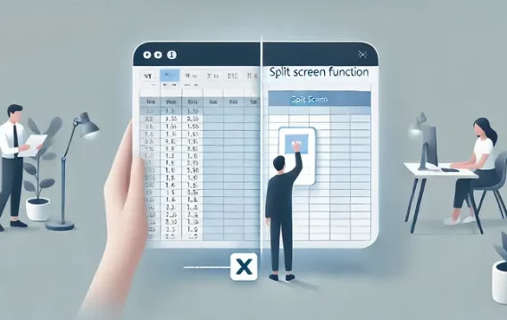
If you are working on a large spreadsheet in Excel, it can be tedious to compare data from different sections.
Is there anything you can do to streamline the process? Definitely, there is – you can use the split-screen function.
What is the split-screen function?
The split-screen function on Excel enables you to view separate sections of a spreadsheet simultaneously. This way, you can quickly compare your data without scrolling back and forth.
How to use the split screen function in Excel?
Excel gives you complete control. You can customize the way the screen is split so as to meet your specific needs.
To access the feature, click on the View tab and select Split from the menu.
To use it, there are several options available to you:
- Split the screen into four equal quadrants.
- Split the screen vertically or horizontally.
Option 1: Split the screen into four equal quadrants
You can split your screen to create four copies of your current worksheet. All the four copies are set side by side so you can view them at the same time.
To achieve this, follow the simple process below:
- Go to the A1 cell and select it.
- Click on the View tab and select the Split option from the menu.
That’s it. Your screen will be automatically split into four worksheets.
You can make adjustments by clicking and dragging the sides of any of the worksheets or the center section.
Option 2: Split the screen vertically or horizontally
You can split the screen in half instead if you don’t require four copies of your worksheet. Depending on your preference, you can create vertical or horizontal splits.
To create horizontal splits, here’s what you have to do:
- Go to the A column and select any cell except A1.
- Click on the View tab and select the Split option from the menu.
The split will be automatically created above the row of the selected cell. For instance, if you selected the A5 cell, the split will be between row 4 and row 5.
Creating a horizontal split is as easy as this:
- Go to row 1 and select a cell from any column except column A.
- Click on the View tab and select the Split option from the menu.
Once you have selected any cell and clicked on the Split button, the spreadsheet will be split. But you need to remember that four quadrants will be created instead of two when you choose cell A1.
How to remove the split screens?
When you are done using the function to compare sections of your spreadsheet, click on the View tab and select the Split option again to turn it off. You will have a single worksheet again.
Alternatively, you can disable the feature by dragging the split screen bars to the edge of the window.
There you have it. You’ve discovered how to make your work easy by using the split-screen function on Microsoft Excel.
It’s important to keep your PC running smoothly if you wish to complete your work without any hitch. Some users experience annoying system glitches and crashes while trying to get an important assignment done.
If you are facing such issues, use Auslogics BoostSpeed to perform a full system checkup. The tool is very user-friendly. You can schedule automatic scans to locate and eliminate junk files and any speed-reducing issues that may be causing your applications to hang. It also includes a privacy protection feature to safeguard all your sensitive personal information while you surf the web.
We hope you’ve found this content useful.
We’d love to hear your thoughts…
Feel free to drop a comment in the section below.
